
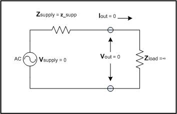
Figure 1: A Basic General HDS Device Model
Hybrid dynamical systems are defined as a finite state machine (FSM) and a collection of dynamics models. The FSM state determines which dynamics model is "in control" at any given time.
This document points out a few of the problems encountered when applying this simple form to general models, and suggests techniques for making the models far more useful. Some of the main interests of the efforts related to this project are to be able to recognize criticalities, and the inputs and internal behaviors that can cause various types of behaviors. It also aims to enable monitoring observable outputs and differentiate actual and likely failure modes as opposed to the proper behavior of the modeled component.
The main thrust for this project includes using the HDS models for each component in a network rather than using a single aggregate model for the entire network. This permits creating individual component (node and link) models for unique component types separately. Many of the component HDS models may be replicated for multiple nodes or links of the same component type. The concept of driving point impedance (DPI) is introduced and integrated into the network model approach to allow the component-based HDS models to be easily applied to continuous resource flow networks (such as power flow models) .
It is useful to consider the behavior of each HDS model as following behavior trajectories through a model-defined behavior state space. The limitations imposed on that trajectory due to the limitations of the physical system being modeled can be analytically useful considerations. The trajectories can be shown to have bounded regions of traversal and, once those bounds are defined, the number of combinations of behavior possiblilities that must be considered and modeled may be greatly reduced.
The general HDS model presented above, as with most simple models, has many hidden complexities that usually must be taken into consideration for its practical use. To illustrate some of these hidden complexities and how to handle them the electronic circuit model in Figure 2 is used.

For each of the FSM states the dynamics of the circuit can be defined as follows:
      Zsource = z   the modeled internal impedance.

      Vsource = 0   the voltage for "Down".

      Vout = 0      there is no output voltage.

      Iout = 0      there is no output current.

      Zload = ∞     the unknown external load
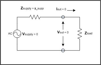
      Zsource = z     the modeled internal impedance.

      Vsource = 0     the voltage for "Down".

      Vout = 0        there is no output voltage.

      Iout = 0        there is no output current.

      Zload = Zextern  the external load (from model propagation)
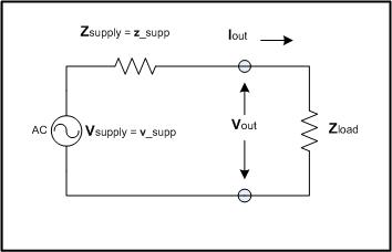
      Zsource = zsupp     the modeled internal impedance.

      Vsource = vsupp     the voltage for "On".

      Zload = Zextern   the external load (from model propagation)

      Iout = Vsupply / (Zsupply + Zload)

      Vout = Iout * Zload
Something has caused the system to act in a manner that degrades its performance. Often there can be multiple versions of this state, which should each be modeled as separate states. It may set the state variables as follows:
      Zsource = zdegraded     the modeled internal impedance.

      Vsource = vdegraded     the voltage for "On".

      Zload = Zextern         the external load (from model propagation)

      Iout = Vsupply / (Zsupply + Zload)

      Vout = Iout * Zload
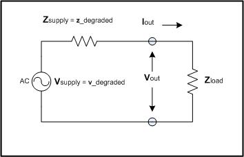
Of course, there can be diffrent types of degradation, and two that are of interest here are changes in Zsource and changes in Vsource. These could be two different types of degaded performance, and therefore become candidates for two separate "Degraded" FSM states.
If the model is made up of many "patches" resulting from different dynamics behavior functions and behavior parameters for each FSM state then the modeler should be aware of each of the following:
What are the "state variables" defined for each of the dynamics and for the overall model, and how are they related, especially for the separate dynamic models for each of the different FSM states?
A single consistent set of "state variables" across all of the dynamics definitions allows the total HDS model to be considered as defining a single state space of the behaviors of the overall HDS model via these state variables. This approach may force state variables from one dynamics model to be included in the overall collection even though they are not used by the other dynamics models. A reasonable way to select and maintain useful values into "unused" state variables is needed.
The difficulty with this preponderance of possibly "unused" state variables is deciding which ones to set and to what values. Is there a need to maintain a "reasonable and valid" value in a variable that is not being used in each dynamics model? This is often made more obvious if the specific transitions are considered, and the variables are selected and values set based on the dynamic models to which the HDS model can transition from any given FSM state. Which state variables contribute directly to the externally observable and output variables must be considered here also.
Are there discontinuities in the values of the state variables as FSM transitions cause the state variables to cross the patch boundaries?
There may be many discontinuities, whether in the base values ("Up" Vsource or Zsource versus their "Degraded" counterparts versus their "Down" values) or any various derivatives in the state variables vector. However, only those patch boundaries which are traversed by defined FSM state transitions must be considered when trying to guarantee model continuity during those transitions.
A physical system, even simply modeled, has a "mode of behavior" for each of the defined FSM states. These modes of behavior are the focus for selecting the states of the FSM, but once identified the transitions between the modes of behavior must be considered individually.
The transitions for this power supply model include:
The transitions can all be modeled as abrupt and severe discontinuities, but that would give uncharacteristically ideal well-behaved but sudden discontinuous changes in both voltage and current. This is impractical for real physical systems and is moderated by the complex variable contributions of system impedances and the actual physical makeup of generators. Another way they can each be modeled is by adding intermediate "transition" states to the FSM, much like the "Init" state described above. Each needed transition would have its own dynamics model for the behavior over that type of transition. These transition dynamics models would, in most cases, have to include a time period for the transient behavior and then, when complete, must trigger an FSM state transition to the originally targeted FSM state.
So, how should the transient behavior be modeled? That depends on the physical behaviors of the modeled component device. When the device is turned on does the power supply gradually increase in voltage, does it spike then drop back to the desired value, or does it have another characteristic behavior trajectory? When turned off does the power supply gracefully slope down to 0 volts or does it display another characteristic behavior trajectory? Each of these transition models must be considered separately if this HDS model is to help identify effects of criticalities on the actual device behavior and its influence on networks which include it.
Without modeling individual device criticalities it would be very difficult to reasonably predict the behavior variations that can cause failures internal to the device or unexpected behaviors that may dominate its influence on other externally connected components.
As discussed above, the HDS model's state space is defined by the number of state variables that must be included in the overall HDS model. However, there are wide regions of that space that are not realistically accessible for traversal. These restrictions are caused by the following:
There is no immediately obvious way to generate a perfect representation of the many trajectories the behavior of a device may take, but some limitations on specific state variables can usually be guaranteed. This enables defining behavior limit regions and, therefore, the eligible model behavior regions to include and exclude in the model state space.
There are ways to generate many variations on state space behavior regions. A good starting place is to define the behavior limits on the ideal elements of the component model. If the voltage source is either on or off then it is either running in its expected range of output or it is at zero. Investigating the extremes of values possible for the load impedance, which is expected to vary over time, the limits on the other state variables can be estimated. These estimates allow the behavior state space region boundaries to be identified and characterized.
Some preliminary estimates show that if the load approaches z = 0 then the maximum current is given by
Iout(max) = Vsupply / Zsupply
and the minimum voltage from Vsupply is given as
Vout(min) = 0
If z = ∞ then the minimum current is
Iout(min) = 0
and the maximum voltage is
Vout(max) = Vsupply
When these limits are entered into the equations for the dynamics model for "Up" the steady-state behavior is well-defined and has immediately calculable implications on the other state variable values, thus defining a behavior region for the dynamics model. Other,but manageable, implications come from reactive power aspects of the complex impedances.
Due to the capacitive and inductive components of the impedance the above picture becomes somewhat naive, as the sudden changes in voltage or current can induce strong "back-EMF" inducing high voltages or currents as transient behavior caused by the power supply transitioning from one state to another. In power systems an attempt is made to perform the real-world state transitions only at zero crossings of the AC power, voltage, or current, but the timing of failures and spurious incidents is generally not so accomodating. The resulting voltage or current surges can be considered critical in identifying which events may become triggers of failures, especially when they exceed the capacity of a transmission line or the power limits of components attached to the power supply.
Each tolerance limit, whether it is the voltage at which a capacitor fails or the current at which a resistor or wire overheats, becomes a critical limit that should be considered in the behavior region boundaries for the component's state space. Without these details the model cannot anticipate an overheated wire or resistor, and therefore the effects it has on power delivery.
The critical limits may be considered in several categories:
Working from these three definitions five categories of behavior "risk of failure" categories can be defined:
One step to being able to better predict an estimated mean is to use existing stochastic model techniques, such as Kalman filter variations, to maintain estimates of the variations of the values, while periodically updating them to reflect real-world observations when they are available.
To be able to estimate the extents of the probabilistic boundary region about the current mean for a value the model must be aware of the probability distribution function for the variable. When using a model to which Kalman filter variants are applied it is assumed that the variable estimate is from a variable with Gaussian noise added to it. This makes the distribution symmetric and the range of "Probable" values easy to calculate. Another approach to use when the distribution is obviously not Gaussian is to propagate a piecewise linear PDF and calculate the extents on either side of the mean that give the desired probability of inclusion. This result may not be symmetric about the mean.
Using the Gaussian additive noise assumption, and assuming the state values vector time step propagation function is differentiable a Kalman filter variant (the "extended" or the "unscented" version) can be applied to the state variable propagation steps so a covariance matrix is maintained. Using the covariance matrix the interdependence of state variables and the variance of the individual variables can be used for estimating the PDF, and thus the probabilistic boundary interval around the estimated state variable at each step. The result is that any state vector transition between the "critical regions" can be detected and modeled.
There is another advantage to using the Gaussian assumption and the Kalman filter approach. The methods for updating some or all of the state variable values and the covariance matrix from actual observations, also assuming some Gaussian distribution of additive noise, are well defined. The result is that the HDS component model's state variables vector can be propagated through predicted model behavior steps with error estimates, then updated to be brought closer to reality when real-world value observations become available.
By using the HDS model and the model forms outlined above the component models can be easily combined into large models of many components networked together and still retain the needed details of the contributions of the components.
For continuous network flow models of large, sparsely interconnected systems modeled as a single dynamical model or as a single HDS model must be represented by very large vectors and matrices. When matrices get extremely large the operations on them, such as calculating a matrix inverse, get very time consuming and begin to accumulate dramatic computation errors. The calculations can be parallelized to speed them up, but to parallelize the problems to take advantage of parallel processing speedups requires customized algorithms for each computation.
To get away from the programming complexities and grappling with the problem sizes it is recommended that the network be represented by a graph of the network topology, and that each network node and link have associated with it an HDS model. Each node and link represents a component in the network and can be modeled more reasonably as a single, relatively simple HDS model of that component device. This approach introduces some overall model computation complexities, but allows extremely large network flow models to be easily combined from a relatively small number of component HDS models. The approach also allows the models to be easily spread among parallel processors by subdividing the overall network on the identified links, while minimizing the interprocessor communications needed.
Each HDS model need only communicate with those other network components with which it shares a link. This provides a simple segmentation of the problem using the links and nodes, and allows easy partitioning of the problem to superimpose it onto any parallel architecture.
As stated this reorganization does not come without some complexities. Network flow models often include large systems of partial differential equations, and the "feedback" aspects influence the model's behavior. For electrical systems these often include large numbers of "loop-node" equations. Dr. Ruben Kelly of UNM, using ideas from mechanical engineering that date back into the 1920's, devised a method called Driving Point Impedance (DPI) Techniques for Circuit Analysis. The technique is already used for fluid flows, and by extending his DC and low frequency techniques to AC, fixed frequency with phasing, and complex representations voltage, current, and impedances this system approach can be applied to modern electric power systems.
Using DPI a network, from the view of each component, consists of modeling the internals of each component and the driving point impedances from the point of view of each of its connections to the rest of the network. To employ this technique in electric power network flows the overall model must be updated each time step in two phases:
One consolation is that if impedances, voltages, and currents do not change they do not need repropagated. This makes it useful to maintain the DPI value for each portal for each component, as well as a list of voltages and currents from the various contributing sources.
Considering a large network of HDS models some questions need discussed:
When an HDS model is used to model a single device in a large network of devices how many of the state variables need to be propagated to other components of the network?
Only a few of the state variables, or even variables derived from them need to be passed to the neighboring network components. The components themselves will determine which of those need integrated with their own state variables and passed on. A transmission line model may generate a driving point impedance (DPI) value for each of its ends, based on what is on its other end and its own contributions of impedance. A load must present its DPI to each attached transmission line. A transformer must calculate the contribution from the DPI on its other side as well as include its own contributions to the impedance.
How does each component determine what the DPI of the loads it is connected to (driving)?
The impedances must be passed out every link from a node, and may be unique for each link. Only after the impedances have been propagated across the network can the voltage and current contributions be calculated for each source at each component. In Phase I sources have only their internal impedance to propagate, loads likewise, and only transformers, transmission lines and other "inputs to outputs" devices must be able to pass impedances from one side to their other side.
How does the model get the voltages and currents at the various locations in the network?
The DPI allows easy calculation of the voltage at each node due to a voltage source, and the voltages allow the calculations of the currents through each link and load. The current contributions from the multiple voltage sources are added together to get the total currents through the specific components.
How do we avoid needing the loop-node differential equations in these calculations?
The loop-node equations are to compensate for the dynamics of the voltage and current variations of the frequencies involved. For steady-state AC at a fixed frequency these can all be converted to a higher level of abstraction and viewed as RMS voltages and currents with real and complex aspects influenced by the resistive, capacitive, and inductive loads throughout the network. The model can focus on real and reactive power delivery on longer time steps rather than the numerical methods fro solving differential equations which must be run unsing short time steps.
If higher resolution is desired for parts of the network the lower level of abstraction, numerical solutions to the differential equations, are available, but they are not essential for all of the model all of the time.
What other advantages are there of having all these small models rather than a single large aggregate model?
By dividing the network into individually modeled components and combining their interactions via the representative network it becomes easy to
The result is that when the small models are aggregated the criticalities they include can be incorporated into a simpler aggregate model more easily. To generate large aggregate models that are purely linear differential equations many aspects of the criticalities are discarded before the model is built. This prevents the user of the model from even being made aware when a criticality begins to influence the behaviro of the model.
Of course, for criticalities to influence the model behavior the model must be able to detect and respond appropriately to the state vector incursions into the critical regions of the model state space.
Earlier discussions mentioned that some FSM states' dynamics models should be able to run to completion, then trigger an FSM state transition to another state. These states are generally the initialization ("Init") and transition states that should be created to make the HDS dynamics patches "fit together" to form a continuous manifold for the state space trajectories.
In addition to the above dynamics model-triggered FSM transition there are certain internal state variable vector trajectory excursions that should trigger FSM transitions.
At times the internal behavior trajectory of an HDS will cross a boundary into a critical region, whether from normal model responses to changing inputs, or from updates generated from sensor inputs from the real world. These boundary crossings should cause an FSM state transition. If too much current is drawn from the generator and it overheats it can create an open circuit when a wire melts or the internal resistance can rise, causing the generator to operate in a degraded mode. The internally modeled behaviors, as these cases, can cause the actual FSM state transition.
For an internal state variable trajectory to initiate an FSM state transition the condition must be detected, and the state transition initiated. This requires state variable location pattern detection and state transition initiator to be included in the design of the HDS model as in Figure 7.

As indicated in Figure 7, the State Control and Pattern Recognizer is relegated the duty of merging external state control requests with state transitions dictated by internal state variable values' trajectories and critical region boundary traversals.
Even with the pattern recognition, the model is not complete until the modeler realizes that the inputs must go into the proper dynamics model, and the outputs must be generated by the currently active dynamics model. The complete network component HDS model overview is presented in Figure 8 below.

Drawbacks of the simplicity of the basic HDS model were presented, then solutions to each were described. These include the continuity of the "patched" manifold generated by and HDS approach, inserting transition FSM states and creating transition dynamics models to ensure continuity for each FSM transition path.
Considerations needed to include multiple HDS component models in a single network continuous resource flow model were considered, especially the use of driving point impedance techniques to localize aspects generally modeled in global models with global-scope state variable vectors. The resulting network model was then shown to need multiple passes of processing, one for propagation of DPI values, followed by one for propagation of the potential and flow contributions from each source.
It was also shown that using the distributed HDS models and the DPI approach large subnetworks can be replaced by a higher level abstraction, but to generate that abstraction the critical state variables space regions must be propagated into that abstraction. Without those critical regions the abstracted model loses its ability to detect actual, imminent, or likely failures of the system or its components.