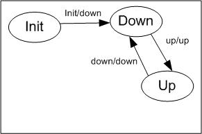
Figure 1: Simple Finite State Model (FSM)
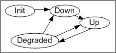
Figure 2: Refined Finite State Model (FSM)
This document presents some concepts whose natural progression in the quest for accurate models of real-world phenomenon and cost-effective "adequate" representations have evolved into hybrid dynamical system (HDS) models and then to multiple levels of abstraction for those HDS models, including the finite state abstraction (FSA).
This document presents the fundamental concepts of dynamic models, then shows how modeling needs made HDS models, followed by levels of abstraction for the HDS model representations as the logical steps to more accurate and computationally efficient models of real world system behaviors.
The components of an HDS model are discussed separately, and then how they are used together to represent more accurate models of complex dynamical systems is discussed.
Early models of dynamic behaviors and physical attributes were often implemented as differential equations and computer implementations of functions continuous over the value ranges of interest. Curve fitting was the method of choice for selecting the "best" model to represent real-world properties and behaviors, but natural deviations from these ideal curves led to "bad fits" of various phenomenon.
These "bad fits" are generally handled in one of three ways: 1) statistical descriptions of the variations, 2) increased order of polynomial and trigonometric interpolators, and 3) increasingly complex differential equations. Once a model is "accepted" the problems these solutions bring with them are ignored until the inaccuracies of their predictions become intolerable to the using community.
For these "accepted" models the statistical descriptions of the variations in the "error" are assumed to follow a statistical distribution. The distribution is defined assuming the deviation "mean" should be 0, indicating the model is absolutely accurate and all the deviation of the real data from the model is due to measurement error or a noisy signal. The true measured value's deviation from the actual model value is then attributed to the errors in measuring the actual values.
Given these assumptions the distribution of choice is logically chosen via the "Central Limit Theorem" to be the normal distribution. This choice ignores the fact that the measurment devices and signal noise may not include the full range of values possible for a normal distribution (infinite value range tails) and, in fact, are often limited to +/- 1 of the measurement instrument's least significant digit of precision or accuracy and the maximum range of the variations of noise.
At this point the model is assumed to be the accurate representation, and the real world measurements and "noisy signals" are blamed for all the anomalous value variations. Users want to be able to "see beyond" this measurement error and noise. Better measuring devices have been built, and "noise filters" have been applied, but the still unexplained variations often force the modelers to consider new models.
Similarly stochastic representations of the "noise sources" have to be generated to handle the widely varying differences between smooth predicted values and actual measured values. Fractal estimators were invented to characterize the "roughness" of the variations. These estimators often need to vary over the spatial and temporal "regions" of the state vector spaces of the model's predicted solution space.
Often to improve the the dynamics or descriptive property models they are "upgraded" to a more complex function which fit the points better. Some fine examples of this include using higher order polynomials or trigonometric sequences to "compensate" for the value deviations from the original model results.
When higher order polynomials and trigonometric sequences are used the behavior of the models between the points often no longer realistically represents what is expected. Further real-world observations often show that the polynomial or sinusoidal trigonometric behaviors, which result in inter-point smooth humps and dips, are NOT representative of the relatively smooth or erratically noisy real world phenomenon.
Another approach to compensating for real versus model errors is to use more terms in the model's differential equations to fit the dynamical behavior of the data point observations to the real-world system behavior.
The differential equations work well for "smoothing" a model's behaviors between sample points, but generally this means that different terms dominate the results over different intervals or regions of the data domains being modeled. This forces the use of more complex differential equations which must be solved for each spatial or temporal step of the model, greatly increasing the computation times for the model.
One commonality of these approaches is that the systems and object properties often exhibite different behaviors over different spatial and temporal domains. A dynamic system, when stimulated, will often exhibit a definite and complex transient behavior, requiring a complex dynamical model to anticipate, and often, between stimulations and after the transient behavior settled down, will finally exhibit a "steady-state" or "typical" behavior.
Often mesh models will be implemented to handle the variations in behavior over spatial domains in models. Some mesh models are then extended to handle transient behavior through techniques which refine the mesh to represent the space in more detail, called h-adaptivity, then remove that refinement as each spatial domain returns to its "steady state" behavior.
A temporally transient response is often handled similarly over time by substituting a more refined model that can represent the rapid changes of the transient behavior, and using a shorter time step size, esentially adjusting the "time" mesh refinement for the duration of the anomalous response, then returning to the original representation to handle the "steady state" behavior.
Each of these model implementation forms involves using multiple "modes" of model dynamics computation and multiple "levels of abstraction".
The "modes of operation" may be viewed as the "states" of the model or model component. By itself a finite state machine is just a set of states and a collection of directed transitions. If it is in state st = A and receives input a it transitions to another state, st = B and emits an output which may or may not be unique to that transition. The states and transitions are easily represented as a directed graph with the states as nodes, and the transitions as directed links. The FSM's behavior is then totally defined by the graph, the inputs that trigger each transition, and the output generated by that transition.
Figure 2: Refined Finite State Model (FSM)
Given the above refined FSM (Fig. 2) the transition links may be fully defined by the table below.
| "from" state (st - 1) | input | "to" state (st) | output (mt) | Description |
|---|---|---|---|---|
| Init | "init" | Down | Down | Initialialization |
| Down | "up" | Up | Up | Coming back into full operation |
| Up | "degrade" | Degraded | Degraded | Not up to par |
| Degraded | "up" | Up | Up | Back to full operation |
| Degraded | "down" | Down | Down | Finally finished failing |
Table 1: State Transitions for FSM
As the FSM is "triggered" with new inputs, and transitions take place the actual state of the FSM traces a "state trajectory" of sucessive state values, st, one value for each time t, each representing which state it was in at that time.
| Time of Event | "Move to" State |
|---|---|
| 0 | Init |
| 2 | Down |
| 3 | Up |
| 25 | Degraded |
| 28 | Up |
| 35 | Degraded |
| 39 | Down |
| 50 | Up |
| 200 | Down |
Table 2: Sample State Trace
A simple FSM as above may be adequate in some situations to represent the aspects expected of the given model's use. However, if more detail is needed in tracking a dynamically changing behavior this is not adequate. For an electric power generator one might want to know what the actual power output levels are or what the voltage levels are over time.
To provide the additional dynamics modeling the FSM must become the controller for a hybrid dynamical system (HDS) model.
An HDS is a composite model of a controlling FSM which keeps track of the current mode in which the HDS is operating, and which uses the mode indication for selecting one of several modal dynamics models.

Figure 3: Hybrid Dynamics System (HDS) Model
Using this representation the dynamics of the modeled system may now be represented by each of several dynamics models, and which model is used at any given time is given by the state of the FSM that controls the HDS. The "state" (st) of the FSM is the "mode" (mt) of the HDS and the selector for determining which of the alternate "dynamics" to apply at any time step.
A sample definition for the "dynamics" of the above HDS representing a simple DC power source and the internal system dynamics state variables V for the voltage and P for power being supplied may be modeled as simple as:
| State (Mode) | Dynamics Model |
|---|---|
| st = mt = Down | Vt = 0 Pt = 0 |
| st = mt = Up | Vt = 120 Pt = 1000 |
| st = mt = Degraded | Vt = 100 Pt = 100 |
Table 3: Dynamics Models for an HDS
For the above HDS the dynamics models generally include a set of dynamics "state variables" (Vt and Pt) which represent the values of needed parameters for the model and for the application which is using the model. The entire "state" information of the HDS model includes the current state of the FSM as well as the state variables for the dynamics models, represented by
HDS_Statet = {st, Vt, Pt}
Of course, the above model isn't realistic for several reasons, including:
For the support of dynamics which are influenced by external values the HDS model needs to be able to support external variables, such as dynamics state variable "inputs", along with its set of "internal" state variables, just as the above model needs the impedance into which it is supplying power [1].
These additional external "state" variables for the network neighbors may be used as "input variables" to extend the "state vector" of the HDS. The full HDS "state vector" then includes:
HDS_Statet = {st, Vt, Pt, Lt}
Which allows the dynamics to be responsive to the external influence of the current load value for the DC source:
| State (Mode) | Dynamics Model |
|---|---|
| st = mt = Down | Vt = 0 Pt = 0 |
| st = mt = Up | Vt = 120 Pt = Vt^2 / Lt |
| st = mt = Degraded | Vt = 100 Pt = Vt^2 / Lt |
Table 4: Improved Dynamics Models for an HDS
When multiple dynamics models are include in an HDS model some concerns may come up about their behaviors, especially continuity on the "boundaries" when switching modes. Likewise, multiple HDS models in a collection that have regions of behavior that are well-behaved and easily modeled may be represented by an aggregated HDS model. Collections of HDS models may be embedded in a higher level structure, defining a model of a dynamic subsystem. Such standardized infrastructures can then be used to coherently build extremely large and complex models without generating a confusion of ad-hoc relationships.
When modeling HDS model dynamics the resulting dynamics collection forms an N-dimensional manifold from a collection of (hopefully) non-overlapping "region patches" covering the state space for the model. As such the patches, when taken together, make up the entire space over which the dynamic behavior is to take place. There are some properties which are essential to creating "smooth" models.
The dynamics, taken together, must be continous for many applications. This generally is in reference to the possibility of discontinuities at the boundaries between patches, but should generally be considered within the bounds of each patch also. Singularity points are also of interest here.
However, if it can be shown that the state transitions form a trace line, swath, or are confined to regions that satisfy continuity that can be adequate.
The dynamics, taken together, may need to be continous in the first 1, 2, or up to n derivatives, ensuring "smoothness" for many applications. This also generally is in reference to the possibility of discontinuities at the boundaries between patches, but should generally be considered within the bounds of every patch also. Singularity points are of interest here also.
However, if it can be shown that the state transitions form a trace line, swath, or are confined to regions that satisfy the continuity of the derivatives that can be adequate.
Singularity points and discontinuities both define "critical" points or regions which, if the model ever moves onto those locations it will fail to give useful results.
To explicitely confirm the above criteria list it is useful to be able to characterize the state space "regions" that may be traversed or traced for each mode of operation for the HDS dynamics. By taking an HDS in isolation it may be practical to numerically explore its space and boundaries for each mode of operation if the above cannot not be confirmed analytically.
Simulations may include millions of HDS model instances. When this is the case the models may be distributed over many processors, all working in parallel. Even so, when large groups of the models are modeling aspects of the real-world system that are deemed "incidental" the models may not need to portray the real systems they represent in nearly their fullest detail. At the same time those models on which the user is focussing, even if they represent the same types of subsystems, such as power sources and loads, may need modeled in the fullest detail available.
Sometimes there is concern about including too much detail for the available compute power to handle in a timely manner. If compute power time constraints are a problem then there may be a need for representing and using the models with differing levels of detail for instances of the same model in the different contexts. These "levels of details" are referenced here as different "levels of abstraction" for a modeled dynamical system or subsystem.
A model can be "abstracted" to higher levels of abstraction, as in Figure 4 below, leaving in fewer details (as in aggregating the sources) that must be recalculated each time step, or the model may be "refined" to lower levels of abstraction, giving greater detail and usually employing more computationally intense algorithms. By selecting different levels of abstractions for different parts of a simulation the user can easily reach a balance of less detail in areas of lesser interest versus more detail and accuracy in areas of heightened interest. By varying the level of details the user may minimizing the required compute power to get their analysis done.
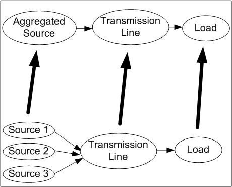
Figure 4: Network Abstraction Levels
The above power source system could be modeled in even greater detail by assuming it is a set of batteries and modeling the details of their internal chemical activity, modeling the effects of heating and electrode aging on its performance parameters, and modeling the changes in internal resistance. However, some of these minor details and their effects may not be useful in a specific application and may therefore be abstracted away in those applications.
One derivation of a high-level abstraction is to create some extra FSM states to represent "fuzzy value combinations" for the externally significant state variables, eliminating the actual state variables completely. This is one way of creating a finite state abstraction (FSA) for an HDS. The FSA represents the HDS adequately for certain types of analysis, and replaces the HDS with only a single FSM and no dynamics calcuations.
When changing levels of abstraction in a model consideration must be made to which internal state variables are shared for use by "neighbor" models, and the abstraction used must provide a reasonable value for each shared state variable. In many cases this may mean that a constant is stored into that state variable and never changed, and in other cases it may mean that a simple dynamical model may be required just to provide a useful change in that variable's values.
When used in aggregated collections of HDS models it is sometimes useful to create a single HDS model abstraction for a subset of HDS models whose current behavior is steady-state, or appears constant to thie neighbors. Such aggregated HDS models are actually just an HDS model which has simpler dynamics, and if inputs come in that would prompt the contained HDS models to begin a complex transient response the contained HDS models can be activated as one mode of operation for the aggregate HDS model. The aggregate HDS model must be responsive to EVERY input that would otherwise be used by the contained HDS models and present a response to every change on those inputs which adequately conforms to the response of the collection of included HDS models.
The HDS model form defines a framework providing a standardized structure for models of complex dynamical systems. It provides for a complex dynamical system model, whose dynamics must operate in many modes, a versatile representation. It allows easy model modification for refinement or generating simpler abstractions. The HDS model framework helps the developer to organize the modeling clutter formerly generated by the common ad-hoc approaches used for organizing dynamical models. By putting dynamical models into the HDS model framework creates easy model building blocks. Each block may be instantiated many times in a single simulation, they may be abstracted to any of a number of levels of abstraction, and they each become a single unit model for independent validation.
Similarly, dynamic models are often combined in an ad-hoc manner, causing large complex models to become extremely difficult to understand, maintain, or update for expanded or new domains being modeled. The versatile HDS model building-block form may easily be put into a structured form, such as a mesh model or a network flow model. By putting multiple instances of basic HDS models into either of these structured forms the combination becomes a single higher level system which may include extreme complexity and detail.
This modularity and structure of model design makes the resulting models easy to understand and maintain, and provides standardized conventions for building and combining many models into even larger-scoped models. This approach is commonly used for modeling electronic circuits, but is not common in other network-based models.
Using the HDS model building blocks and mesh or network model structures extremely large models can be built which define the aggregate dynamics of complex systems. These model dynamics can then be included in an aggregate HDS model as one of its dynamics models for a single mode of operation. The aggregate HDS model then represents a high level building block, itself composed of lower level building blocks. This defines a hierarchy of models.
The result of building a hierarchy of these models is to provide a clear and practical approach for incrementally generating high level models of far more complex systems of systems that can be used in scalable environments.
The hierarchical model form above may be used in a highly parallel environment so the lowest levels of representation may be modeled over the entire system. The same model may be used in a resource-starved computing environment, such as on a laptop, using higher levels of abstractions, and thus simpler models, for all the periphery details, while expanding the detail in only those parts of the system that require close examination.
A modeler may use the HDS model form to generate simple encapsulated model forms for the dynamics of any system. The HDS model may be abstracted to run faster and provide less detail, or it may be refined to provide greater detail.
Combining HDS models with a mesh or network flow model allows organizing a large number of dynamical component models into a dynamical system model. Such dynamical system models can then be combined into even larger system models while retaining a strict hierarchical organization.
Using low levels of abstraction, providing the maximum details provided by the model, the HDS models may be distributed onto many parallel processors to provide detailed model projections. By using high levels of abstraction, minimizing the detail to reduce the model sizes, the HDS models may be reduced to run in computing environments with minimal resources. Even the reduced HDS models may be selectively replaced with refined models allowing details of concern to be more accurately modeled.
This a graph whose links are all directed from a "start" node to another (or the same) "end" node. If a link is required in the other direction it is represented by another link directed from the second node back to the first.
For the purpose of this paper the dynamics of an HDS (hereafter just called dynamics) are the collection of algorithmic models which propagate the current (and possibly previous) values of the HDS state variables into the next time step's values for those state variables.
A finite state machine that replaces an HDS by representing its dynamical state values via a "fuzzy variable" mapping, such as "high", "medium", and "low" states rather than the dynamical model's representation of continuos-valued variables. This may also involve enumerated patches for N-dimensional "regions" of a spatial "volume".
The FSM consists of a collection of "states", and a definition of transitions among those states, defined by a quadruple including
The FSM can only be "in" one state at a time, and the "from state" and input combination must be unique for the FSM's transition model.
The FSM is commonly represented as a directed graph where each node represents a "state" and, by necessity, consists of a single connected graph "component". Since a single node may have multiple transitions to any other given node, triggered by distinct inputs, the graph may have many links between any two nodes.
This is a mathematical construct defined by a set of nodes and a collection of links between pairs of nodes. A graph is connected if there is an undirected path from any node to any other node. If there is no such path for any single given pair of nodes then the nodes belong to separate components (disconnected subgraphs) of the graph.
These are the variables which, in dynamic modeling, represent the "state" of the system being modeled and, in physical system models, may include such things as a particle's position, velocity, and accelaration vectors, mass, temperature, volume, surface area, number of contained items of interest, or stress tensors. Any variable essential to the dynamical model and/or its interfaces to other dynamical models may be considered state variables.
An HDS is a model made up of two parts, a Finite State Machine (FSM) which controls the model's "modes of operation", and a collection of alternate dynamical models, which includes a collection of dynamical state model variables.
The FSM is defined above, and its "states" are mapped to "modes of operation" for the for the HDS. Its "mode" determines which alternate dynamical model is to be applied to the dynamical state model variables.
A mesh model is generally a spatial model which divides its spatial domain into many regions which are then modeled as separate but "neighborly" entities. Each region has its own internal state variables and dynamics models, and accesses some state variables from its neighbors as inputs.
A network flow model is a logically connected graph model which has state variables and dynamic flow models associated with each of its nodes and links. These components are then modeled as separate but "neighborly" entities. Each component has its own internal state variables and dynamics models, and accessing some state variables from its neighbors as inputs.
A path is any sequence of links between two nodes of a graph, where the successive links share a common node and form a sequence from the first "end" node to the other "end" node. Traversing a path involves following an alternating sequence of node, link, node, link and ends on the final "end" node. A directed path involves only links that are directed from the node that precedes its occurrance in the path to the node that follows it in the sequence. If any links are reversed it is an undirected path.
A subgraph is any subset of the set of nodes in a graph, and may include none, any, or all of the links between the pairs of included nodes.