
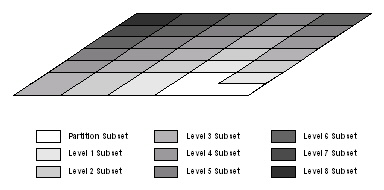
Figure 1: Sets, Relations, and Fields Example
2010-11-11
James R. Holten III, PhD
Institute for Complex Additive Systems Analysis (ICASA)
New Mexico Institute of Mining and Technology (NMT)
Socorro, NM, 87801
This paper describes how the concepts of the SRF Algebra may be applied to define the steps needed in partitioning a large data model and to generate the communications maps needed to effectively pass the necessary data between process partitions. Using the partitioning and communications map descriptive metadata the paper also shows how the various load types: processing loads, partition sizes, and communications loading, may be included in the partition assignments decisions. The algorithms defined via the SRF metadata is then easily converted directly into code to perform that partitioning and other defined operations on any application represented using the SRF data model. The partitioning is generalized, and allows any number of partitions. The approach itself is being parallelized for use on exascale HPC applications.
The SRF (Sets, Relations, and Fields) Algebra [1,2] was devised as an metadata abstraction for basic data_model representation and manipulation. The abstraction provides a standard for a simple description of data object collections. The descriptions, in turn, enable expressing the data object interrelationships, data structure algorithm operations on those data objects, and data structure related analysis steps. The basic representation of data relationship allows concepts and data objects from one application domain to be easily shared by developers and analysts in other application domains. The abstractions also allow merging the data structures and data relationships of multiple diverse models into a single application code. Models and programs developed using the abstractions of the SRF Algebra have been built, and those implementations demonstrate how data and analysis tools can be easily constructed to be shared among diverse application codes.
SRF models have been generated for generalized mesh models, finite element mesh models, molecular models, particle models, and generalized network models. The concepts and algorithms presented in this paper may be applied to SRF models of any of these forms.
This paper presents how to apply basic parallel partitioning concepts to SRF-based model descriptions for easy conversion to data-parallel constructs for an arbitrary number of processor partitions, and can include model element and partition weighting calculations for estimating partition data sizes, processing loads, and communications loads for load balancing across the process partitions and communications channels.
To enable sequential programs to be scaled up to handle extremely large problems the programs must have their data partitioned and parts of the data assigned to each of the allotted processors for parallel execution of their algorithms [6,12]. The complexities of partitioning data for extremely large and complex problems so they can be ported onto parallel architectures cause many model developers to fall back on the old standby approach of using structured (usually rectangular mesh) models and dividing the problem by an integral number of segments in each dimension, generally via recursive coordinate bisection (RCB). These choices force the partitioning to be dependent on adjacent rectangular blocks of a predefined size and number, and cannot be easily adjusted in size to allow for balancing the computational and communications loads across the processors or communications links. Often this restricts the programmer to assume homogeneous processor and communications characteristics, preventing the use of the partitioned problem on distributed and nonhomogeneous parallel architectures.
Historical efforts have shown that fixed-sized meshes are impractical for many applications, as adaptive mesh refinements (AMR) allow generating finer resolution around "interesting" regions in the model, so overlays of regions of finer rectangular meshes are commonly used [8,12]. Also the rectangularly structured mesh model approach is useless for large-scaled network models such as those needed in modeling critical infrastructure networks using graphs and network flow models. Similarly a more general representation is usually needed for molecular and particle models.
The SRF Algebra [1] is based on abstract sets of objects, fields of properties or attributes for each of those objects, and relations describing the associations between pairs of members of a single set of objects, or between members of a pair of distinct object sets. The abstraction maps easily to collections of objects as class instances, as in C++ and Java codes, arrays of structs as in C code, or the multiple arrays of properties common in older FORTRAN codes.
The basic SRF objects that must exist in most complex data models are as follows:

In the various commonly used model representations much of the information about the object associations is often implicit. It is only present in the code variable references, the indexing into associated arrays of dependent object properties, and the colocation of data fields and methods in struct or class objects. To understand the relationships between various modeled object types one must reverse engineer the intent of the implementer. The data associations intended by the programmer or model developer is often not obvious to the reader from the data organization or from the code unless it is described in comments or supporting documents. Because of this obscurity of intent mistakes are easily made when updating or parallelizing the code, either from simple oversights, not realizing the significance of awkward code, or from gross misunderstanding of intent when scaling the code in these models for larger problem sizes. This can happen regardless of the programming languages used because of the obscurity that implicit relationships provide.
Much of the complexity of of partitioning data onto parallel processors comes from determining which data must be shared between processors. Here a few terms must be defined for the purposes of this paper:


Putting code data models into the conventions of SRF representations makes the relevant data relationships explicit. This paper describes how to utilize these explicit relationships to enable the partitioning needed to scale up the problem sizes, even to exascale extremes.
The metadata abstractions provided by the SRF Algebra data model provide the mechanism for describing the relationship of data partitioning constructs to the parts of the modeled data. In this paper the description of the partitioning is derived, then it is used to describe the creation of communications maps. Once the partitioning and communications relationships are derived and presented methods for calculating loading estimates and comparing limitations relative to assigning partitions to system resources (processors and communications links) are discussed.
In this document, when an expression is derived that can be generically applied to any of the element types above, the generic E will be used instead of repeating the derivation for each of me, se, or te element sets.
There are generally two types of data passing steps for which data sharing patterns must be considered. One is at each time step, and the other is on each iteration step for some iterative operations within a time step. Also, the complexity of generating sharing maps can be amplified by having different elements use different time step sizes. This paper focuses its efforts on the basics by assuming only fixed time step sharing is needed, however the derived procedures may easily be applied to the other sharing type and nonhomogeneous time step sizes as well.The "Partitioning Elements" section describes how the partitioning of the major elements is projected via composition of relations to the other model element types, and how those projections identify which elements must have their field values shared across partition boundaries. It also defines which partitions in a partitioning of the model must communicate (share data) with which other partitions.
The "Communications Maps" section shows how ownership of an element indicates which partition does the calculation of values for that element, preventing one category of potential race conditions. This also resolves which are the partitions with whom the calculated values must be shared. It then shows how the ownership and sharing can be converted to identify, in detail, which elements' field values must be communicated to each of the partition's "neighbors".
The "Calculating Loads" section describes various methods for describing loading through calculating partition data sizes, partition computation requirements, and communications link transfer volume needs. It then discusses how any given configuration of element ownership by the partitions, through the use of the partition relations and the communications maps, can estimate those expected loads for each partition and communications path. Once these load types are discussed methods of "load shifting" to create a more load-balanced assignment of elements to partitions are also discussed.
The final section discusses a collection of applicable concepts and techniques, including
In order to allocate parts of a large data model onto multiple processors and coordinate the activities on these processors the developer must be able to partition the data for data-parallel processing. The developer can then use that partitioning and the data element type interdependencies to determine what to communicate between each pair of processors.
The first step in dividing the data elements among the processors is to create a set of partitions, with one partition for each processor. Then by assuming that an assignment of the major elements to each processor partition can be made, the needed data model manipulations can be defined. The partitioned major element to partition assignments are represented by the following:
The first step in partitioning the data involves getting the element members that are the contents of each partition for each element type. This is done by using the relation compose operations to project the partitioning of the major elements onto each of the other element type sets in the data model.
As shown in Fig. 4 above, each partition must include its owned major elements and the full contents for every element type on which the calculations for these major elements' field values depend. The contents of the partitions also need to be broken out into categories of private; pass (owned and shared ); or receive (being not owned, but needing shared) from other partitions.
The major elements that must be present in each partition may be limited to the above owned major elements. A common case however is, while computing field values for a given major element, access to values from "neighboring" major elements is needed, defining a ghost region of major element data, as in Fig. 5 above, that must be copied to the local partition. To use ghost regions the full collection of major elements present in each partition must include those receive neighbor major elements also. The full collection of major elements that must be represented in each partition may be generated via whichever of the following applies to the given model implementation:
Once the major element ownership assignments are made they can be "projected" via relation composition to the other element types, getting the full list of each element type that must be represented in each partition as follows:
To understand the computational needs of each partition and to generate communications maps among the partitions it is still necessary to know which elements are "owned" by each partition.
Once the relations above describing the associations of each element with one or more partitions have been calculated many of the member elements in the relation RE,p should reference only one partition. By assigning the ownership of those elements to that one partition any possibility of their associated field values needing passed between partitions is eliminated, greatly reducing the amount of inter-process passing of element data needed.
The three categories of ownership relations needed for each partition, private, pass, and receive, define independent subsets that cover the full set of members of the partition. The last two, pass and receive, define the elements that are in each partition's share subsets, also known as the "shadow regions" illustrated in Fig. 6 above.
The ownership is uncontested for the private set members, and they
do not need their attribute field values communicated. These private
members can be represented in the subset given by those element set entries
with only one partition range set reference. Using the generic E, as
this must be done for each element type, a field of boolean private
flags (Fprivate,E) can be derived, then the field values
can be used to define the subset of elements that are private for each
partition as follows:
Fprivate,E =
(FieldOf(RefCounts(RE,p)) == 1)
Then the members of SE that are private in any partition
are identified as a separate subset of SE via
SE_private =
Subset(SE,
IndexTrue(Fprivate,E))
and its subset relation (which enumerates the parent members in the subset) is
given by
RE_private,E = SubsetRel(SE_private)
The relational mapping of the private elements to the owning partitions is
then derived as
RE_private,p = RE_private,E *
RE,p
The actual indices in the global element set SE of these
private members of each partition may be enumerated via the composition
which remaps their subset indices to the global indices as
RE,{private},p =
RE_private,E-1 *
RE_private,p
The private global set member contents of each partition may be listed
as the references of a mapping from the partitions to these members via the
inverse
Rp,{private},E =
RE,{private},p-1
At this point it is useful to identify the elements that are shared by
two or more partitions also, but these are just the members of each partition
that are not private, and are given by
RE,{share},p = RE,p -
RE,{private},p
or, the convenient inverse that maps the parttions to their shared global
element set member indices
Rp,{share},E = RE,{share},p-1
The ownership of the shared elements is significant in determining which
partitions are to calculate the elements' field values. Choosing this
ownership also determines to which partitions those values must be passed.
At this point any assignment of the shared members of all but the major
elements to any one of the partitions that shares it can be made. Only the
abstraction for that ownership of the shared members is needed here. The
passing partition relations are identified as
RE,{pass},p
with
Rp,{pass},E = RE,{pass},p-1
Also at this point the full ownership mappings for each of the element types to the partitions can be generated as
At this point the elements whose field values must be computed in each partition are now known, and the computation load for each partition can be estimated. This is done in the later section, "Computing Loads".
Using the above relations for the various sharing and ownership assignments the communications maps may now be generated.
Once the ownership of each element is known the actual communications needs for each element type's shared data can be derived. The communications maps that must be generated for each partition include which elements are to be sent to and received from each other partition for each element type. This allows the shared elements' field values that are to be shared to be passed from the elements' owning partition to their receiving partitions. The "passing of an element" in this context actually indicates the need for passing those property or attribute field values that change over time for those elements that must be shared, even though many parallel models pass all the field values associated with those pass elements.
Communications maps consist of the following details:
The pass elements' field values must be passed to other partitions after each calculation, and each partition's process must know where to pass it. Then each partition must expect to get its receive elements and know which elements are to come from each other partition. Once these are determined then the elements in each message block being passed between a pair of partitions can be determined.
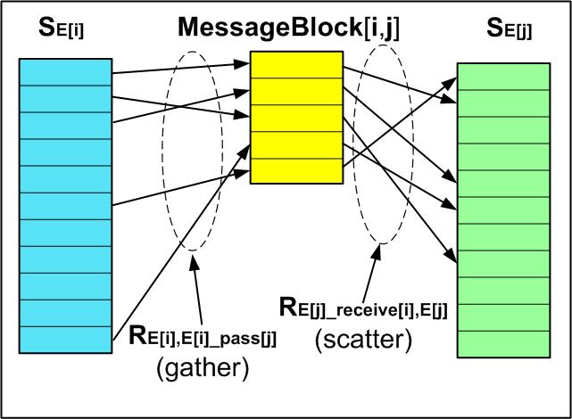
Deriving the mapping of elements to be passed from partition i
to partition j is a matter of finding the passed element members
in SE[i]_pass that are also in
SE[j]_receive, by matching their global
SE member indices.
SE[i]_pass[j] =
SE[i]_pass ^
SE[j]_receive
which is a subset of SE whose elements are enumerated in the
subset relation given by.
RE[i]_pass[j],E =
SubsetRel(SE[i]_pass[j])
which defines the global member indices to be placed into the message block
that is to be passed from partition i to partition
j and therefore is also the subset (and ordering) to be
expected to be received from partition i by partition
j with the content ordering defined by the subset relations
RE[j]_receive[i],E ==
RE[i]_pass[j],E
and the message block set is defined by the subsets, as their size and
and parent set member reference orders are the same, with
SE[j]_receive[i] ==
SE[i]_pass[j]
Once these are found then the subsets of elements in each partition that are to
be included in the message block for each receiving partition can be found.
The local "gather" mapping is merely the mapping of the pass message
block contents to the local element indices in the order the members
occur in the message boock as
RE[i], E[i]_pass[j] ==
RE[i],E *
RE[i]_pass[j],E-1
and the local "scatter" for extracting the member values into the receiving
partition is given by
RE[j], E[j]_recieve[i] ==
RE[j],E *
RE[j]_recieve[i],E-1
These allow the ordered mapping of the partition i element
members' field values to be gathered into a message block in partition
i, the block to be transferred to partition j,
then the message block contents scattered into the corresponding fields for
the correct element set members in partition j.
Each element type's shared members mappings can be used to generate a
relation mapping from the partitions through the shared subsets to other
partitions that share those elements. Using the generic element designator
E the following should be repeated for each element type to get the
partition to partition links for them:
Rp,{E_share},p =
RE,{share},p-1 *
RE,{share},p

Loads on each partition may be estimated for each of three criteria, space requirements, computational time, and communications time.
To estimate loads on the processors, both size and computational,the number and types of elements in each partition must be known. This is given by Rp[i],E for each element type over the ith partition, given by the derived sets SE[i], for all i in [0, Size(Sp) - 1].
The space loading is generally considered an absolute limiting factor, and is not considered in rebalancing unless the space requirements for one or more partitions exceed the available space threshold for that partition's processor. Of course, when adaptive mesh refinement (AMR) [8] is performed dynamically this can be a concern each time step, as the number of elements may change that often. For the purpose of this paper the static size case is considered, but using the approach in this paper this can be easily extended to be recalculated each time step or as mesh refinements are added or removed.
Computational loads and communications loads are often specified via the time to perform the needed task. These are often directly measured, then the measured time values are used to predict future expected loading. They may also be directly measured, then normalized by the architecture-relative performance details. Architecture performance details are converted from times to performance factors by dividing the measured time of performance by the amount of data processed or communicated during that time. This normalized performance factor may then be used to scale other loads for estimates of the comparative performance of the code processing or communications times on nonhomogeneous environments.
In most models the amount of space that is taken up by each element type can be
considered fixed, so the space loading for each partition can be easily
calculated via
E_count[i] = Size(SE[i])
and computing the size of each field over that element type
Fj, E[i]= GetField(SE[i],
j)
field_size[j, i] = E_count[i] *
ValueSize(Fj, E[i])
giving the total fields size, the dominant contributor to the model size in
the partition, for that element type in that partition as
E_fields_size[i] =
∑j(field_size[j,
i])
Then, by summing over the various element types the total model size for the
partition and its numbers of element members can be estimated as
total_size[i] = me_fields_size[i] +
se_fields_size[i] +
te_fields_size[i]
Of course, there is also the space needed for buffers for composing message blocks and the fixed overhead of the problem metadata to be considered, but these are often small and fixed, making them less significant than the model element count dependent sizes included above.
The computational load quantity may be estimated for each partition by estimating the computational load for each field that must be calculated. This loading must include accessing the field values that must be used in those calculations, usually through indexing into arrays. The above model manipulations allow easy estimation via any one of the following computational load estimation approaches:
Of course, for nonhomogeneous processors the directly measured times in the three "loadings" above must be "scaled" by the comparative speeds of the processors before they can be meaningfully adjusted for moving loads between processors.
Communications over a single homogeneous interconnection, such as a common ethernet, forces all communications loads to compete for the common bandwidth. Such shared bandwidth can cause many processors to sit idle while waiting for their opportunity to communicate their data message blocks. Generally some way is considered for separating the communications into multiple channels to reduce the competition for communications bandwidth to reduce these processor wait times.
Often parallel and distributed processes use separate communications channels shared among isolated processor groups, even just point-to-point communications between processors. Of course, this requires that other channels be available for communicating outside the dedicated communications groups.
Since all communications between processors above is defined as single partition pair message blocks then it defines a simple point-to-point communications pattern. Using an overlay of the point to point partition communications links onto the desired communications interconnect architecture and any "transmission layers" which moderate sharing and routing of messages can allow a wide variety of matchings of the needed point-to-point channels and the capabilities of the communications architecture topology.
One criteria that should be observed to minimize communications needs is to assure that major elements found to be "adjacent" via the dependency links calculated above are kept together in partitions as much as possible. These "adjacent" major elements generally define the locality of needed communications, and by grouping them much of the data sharing is kept inside the partition, rahter than forced to cross between partitions.
For this paper only the simple point to point interprocessor communications loading is derived, but methods for extending to more complex bandwidth sharing configurations are discussed.
The communications links must pass the message blocks described above between processes. The form of communications link can greatly affect the bandwidth that is available, and the maximum bandwidth of each link determines the time in which a given volume of message traffic can be conveyed.
The global inter-partition communications link needs are given by
Rp,{receive},p =
Rp,{pass},E *
Rp,{receive},E-1
defining the links for the graph of partition to partition communications that
are needed. This is the point to point topology that must be overlayed onto
the hardware architecture's available communications link topology.
The next step is to estimate the quantity of message load that must be conveyed
over each of the links above. First, a relation set is defined over the
tuples of the above communications graph links relation. This allows the
creation of a field of communications load values to be accumulated as
the message block sizes are calculated for each link. Second the message
block sizes for each communications link are added to the proper entry in the
communications links loading field. From above the number of elements for
each element type that must contribute their changed field values to the
message block are identified for each partition to the ith
partition by Rp,{pass},E[i]_receive which allows
the extraction of the elements for a single element type and partition to
partition (k, i) link by
Rp[k],{pass},E[i]_receive =
Extract({k},
Rp,{pass},E[i]_receive)
and the number of elements in the message block to traverse from partition
k to partition i is
E_count[k,i] =
Size(SE[i]_receive[k]
Once the elements for a given element type that contribute to a given message
block are identified then the message block size can be estimated by adding
the field value sizes for those fields that must be passed. Only those fields
that may change values each time step need be included, giving, for each such
field (indexed by j) over that element type
Fj, E[i] =
GetField(SE[i], j)
The total message block space it requires is given by
field_size[k, j, i] =
E_count[k, i] *
ValueSize(Fj, E[i])
and the total message block space required for all the fields that must be
passed for the given element type is given by
E_fields_size[k, i] =
∑j(field_size[k,
j,
i])
Since the element data for all the element types that must be passed over that
link may be more efficiently passed as a single message rather than separate
messages per element type the total message block size becomes the sum of
the E_fields_size[k, i] values for each of the
element types.
This model enables much more complex variations on the communications load
estimates because once the loading for each point to point link is calculated
they can be combined when message block partition links must share a physical
link, getting the total block size loading for each physical link during each
time step data transfer.
Load shifting is essential when space limits are exceeded in any partitions, and is extremely useful when the computational and communications loads differ greatly between partitions.
Initial load shifting may be done to better balance the initial distribution of elements among the partitions and to compensate for processor and communications link performance variations. In many applications this may be the only time load shifting is needed.
Other applications may have computational loads which change over time or may use AMR at run time to refine specific regions of a model over time, increasing or decreasing the number of elements in some partitions, and thus also the computational and communications loads for those processors. Dynamic load shifting is done during the program run to compensate for these run-time load changes. Dynamic load shifting can be done similar to initial load shifting, but it is useful to estimate actual loading each step and only adjust the element allocations when the load differences exceed some reasonable problem-dependent threshold.
It is obvious that the major elements which need to be shifted should come from among those that are in the share category or, if there are none in that category, then major elements that depend on shared elements of other types, indicating they are near the boundaries between partitions. Moving these major elements between partitions will require moving other secondary and tertiary elements between the partitions also, requiring the accompanying adjustments to the impacted subset memberships, mapping relations, and loading parameters derived above.
If the partition that is overloaded is not a "neighbor" (in the communications topology graph defined by Rp,{receive},p above) of the underloaded partition to which load must be shifted then it is useful to generate a "path" of successive element shifts to handle data migrations gracefully. Such multiple-partition load shift repartitioning is handled easily via the above methods.
Two major concerns have been voiced over this approach to parallel partitioning:
To handle exascale model partitioning the model element set sizes and the relations that must be manipulated can become quite large. To handle the extremely large partitioning problem the SRF algorithm implementations parallelization is being designed and implemented.
Many simulations use rectangular mesh models for their simplicity and ease of understanding. However, the rectangular structure itself uses implicit data element relationships to maintain that "intuitive feel". Adjacency of elements is implicit in that the code merely increments or decrements an index for the neighbor's indices, and if the index goes beyond 0 or some maximum value the indexed element is on a boundary. Both the adjacency and the boundary-ness are implicitly "disguised" in the mesh structure, but define the relationships of "adjacency" and the dependencies of calculations on these adjacent elements' values.. Similarly the associations of major elements to minor elements is often based on some basic index manipulation, because the arrays they are stored in are not of the same dimensionality. Often there must be separate arrays of faces or edges, one for each orientation. These implicit relationships are well understood and easily map into the explicit realtions needed for the SRF representation.
All of these implicit relationships constrain the partitioning of the models onto parallel architectures except in specific index-range based subsets of elements. Due to the complexities caused by the form of the impicit relationships it is even more difficult to use irregular numbers of partitions, shift arbitrary elements from one partition to another for load balancing, or easily generate communications maps for such model variations. Once the problem is expressed in the expicit form of the SRF algebra these variations on partitioning are no longer obstacles requiring ad-hoc workarounds.
Exascale parallel partitioning of extremely large models require that the partitioning problem itself becomes extremely large. The SRF algorithms are currently being parallelized for handling excessively large problem data. An exploratory effort is considering "bootstrapping" an implementation of SRF that is described in SRF iteself.
Also, exascale parallel programs require far more complex communications patterns than terascale problems could use. The complexities of aligning communications maps onto hierarchical communications topologies are relatively easy using the SRF data models and basic graph overlay techniques.
The SRF Algebra is a sets-based abstraction and notation for representing the logical structures of data. By expressing data as sets of object abstractions, property fields over the set members, and relationships between the members of the sets using an algebraic notation gives the designer and analyst a common and logical symbology for tackling otherwise seemingly intractable manual tasks. SRF has simplified the descriptive representations of complex mesh models and the operations needed to perform parallel decomposition and generate the communications maps for the partitioned models. SRF has also been used to represent levels of abstractions for multi-network critical infrastructure models and social networking models. The SRF Algebra is a powerful tool for complex systems modeling and analysis.
The SRF Algebra defines a portable metadata structure in which many diverse model forms may be easily represented, and all the relevant data associations may be expressed in the explicit relations. The sets are simple abstractions for explicitely handling the objects, the fields are just metadata wrappers around the arrays of element property values that already must exist in the models, and many of the relations are just wrappers around association tuples that many models must already store. Only the implit relationships require generating new collections of tuples to make them explicit in the model.
The SRF Algebra abstractions provide the metadata to make explicit most of the relevant implicit associations found in various data models. Levels of abstraction are used to emphasize those relationships that are essential to partitioning the data model and generate the code necessary to scale the code up for substantially larger applications.
James R. Holten III, "SRF Algebra: Foundations", SRFAlgebra_20101116.html 20010-11-11
James R. Holten III, "Sets, Relations, and Fields (SRF) Overview", SRF.html 2007-3-07.
Paul R. Halmos, "Naive Set Theory", Springer, 1974.
Patrick Suppes, "Axiomatic Set Theory", Dover, 1972.
C. J. Date "An Introduction to Database Systems" , Addison Wesley (8th Edition) 2003.
Butler, "SAF Reference Manual", Lawrence Livermore National Laboratory, Jan. 29, 2001.
Larry A. Schoof, Victor R. Yarberry, "Exodus II: A Finite Element Data Model", Sandia National Laboratories, November 1995.
Robert P. Weaver, Michael L Gittings, Galen R. Gisler, Robert F. Coker, Kimberly C New, and Robert M. Hueckstaedt "An Overview of the Los Alamos Crestone Project: Uses for Astrophysical Problems", Los Alamos National Laboratory, AMOS Technical Conference, September, 2004.
Nicos Christofides "Graph Theory: and Algorithmic Approach" , Academic Press, 1975.
Ravindra K. Ahuja, Thomas L.Magnanti, James B. Orlin "Network Flows" , Prentice Hall, 1993.
James R. Holten III, "Parallel MxN Repartitioning", MXNrepartitioning.html 2003-03-18.
Bruce Hendrickson and Steve Plimpton "Tinkertoy Parallel Programming: Complicated Applications from Simple Tools", Proceedings of 10th SIM Conference on Parallel Processing for Scientific Computing, 2001.